Materials+ML Workshop Day 6

Content for today:

• Types of Machine Learning
  • Supervised/Unsupervised/Reinforcement Learning
• Supervised Learning
  • Model Validity
  • Regression, Logistic Regression, Classification
  • Train/validation/Test sets
• Training Supervised Learning Models
  • Loss functions
  • Gradient Descent (if time)
• Application: Classifying Perovskites
  • Installing scikit-learn
  • scikit-learn models

The Workshop Online Book:

https://cburdine.github.io/materials-ml-workshop/

• See the "Introduction" section for intructions on installing Python
• Week 1 content is available for review

Writing Python Code in Jupyter Lab

Installing Jupyter Lab

• Install Jupyter Lab via pip:

pip install --upgrade jupyter

• Run Jupyter Lab

jupyter lab

• Install other dependencies (from a requirements.txt file):

pip install -r requirements.txt

Install Workshop Requirements:

Make sure you have installed the Python packages needed for this workshop:

Copy the command from cburdine.github.io/materials-ml-workshop/ in the Getting Started section.

pip install -r https://gist.github.com/cburdine/.../requirements.txt

Tentative Week 2 Schedule (Option 1):

Session	Date	Content
Day 6	06/16/2025 (2:00-4:00 PM)	Introduction to ML, Supervised Learning
Day 7	06/17/2025 (2:00-4:00 PM)	Advanced Regression Models
Day 8	06/18/2025 (2:00-4:00 PM)	Unsupervised Learning
Day 9*	06/19/2025 (2:00-4:00 PM)	Neural Networks * Juneteenth University Holiday
Day 10	06/20/2025 (2:00-4:00 PM)	Advanced Applications in Materials Science

Alternative Week 2 Schedule (Option 2)

Session	Date	Content
Day 6	06/16/2025 (2:00-4:00 PM)	Introduction to ML, Supervised Learning
Day 7	06/17/2025 (2:00-4:00 PM)	Advanced Regression Models
Day 8	06/18/2025 (2:00-4:30 PM)	Unsupervised Learning
Day 9	06/19/2025 (2:00-4:00 PM)	Neural Networks
Day 10	06/20/2025 (2:00-4:30 PM)	Neural Networks

Alternative Week 2 Schedule (Option 3)

Session	Date	Content
Day 6	06/16/2025 (2:00-4:00 PM)	Introduction to ML, Supervised Learning
Day 7	06/17/2025 (2:00-4:00 PM)	Advanced Regression Models
Day 8	06/18/2025 (2:00-5:00 PM)	Unsupervised Learning, Neural Networks
Day 9	06/19/2025 (2:00-4:00 PM)	Neural Networks
Day 10	06/20/2025 (2:00-5:00 PM)	Neural Networks, + Advanced Applications

Questions about review material:

• Intro to ML Content:
  • Statistics Review
  • Linear Algebra Review

Machine Learning

What is Machine Learning?

Machine Learning (ML) is a subfield of AI (Artificial Intelligence), that is concerned with:

• Developing computational models that make predictions, identify trends, etc.
• Methods that can be applied to improve these models based on data

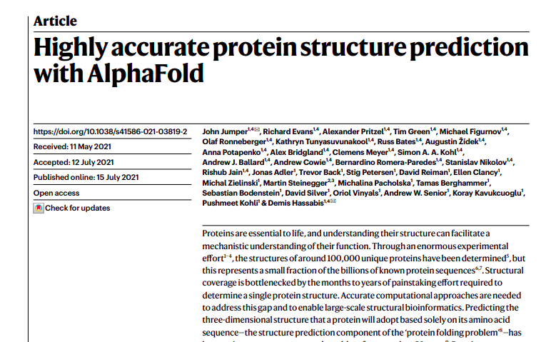
Google DeepMind's Alphafold (2021)

• The 2024 Nobel prize in chemistry was awarded to Jumper and Hassabis for this work:

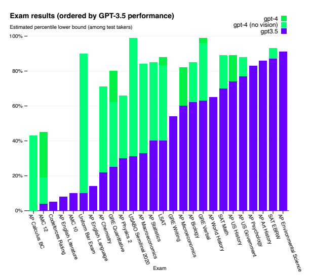
OpenAI's ChatGPT and GPT-4 Models (2023-present):

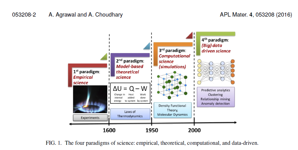
ML in Materials Science:

Types of Machine Learning Problems

Machine Learning Problems can be divided into three general categories:

• Supervised Learning: A predictive model is provided with a labeled dataset with the goal of making predictions based on these labeled examples
  • Examples: regression, classification

• Unsupervised Learning: A model is applied to unlabeled data with the goal of discovering trends, patterns, extracting features, or finding relationships between data.
  • Examples: clustering, dimensionality reduction, anomaly detection

• Reinforcement Learning: An agent learns to interact with an environment in order to maximize its cumulative rewards.
  • Examples: intelligent control, game-playing, sequential design

Supervised Learning

When can supervised learning be applied?

• Problems where the available data contains many different labeled examples

• Problems that involve finding a model that maps a set of features (inputs) to labels (outputs).

• A supervised learning dataset consists of $(\mathbf{x}, y)$ pairs:

  • $\mathbf{x}$ is a vector of features (model inputs)
  • $y$ is a label to be predicted (the model output)

• $y$ values can be continuous scalars, vectors, or discrete classes.

• Here, we will assume $\mathbf{x}$ is a real vector and $y$ is a continuous real scalar (unless otherwise specified).

What is the goal of supervised Learning?

• The goal is to learn a model that makes accurate predictions (denoted $\hat{y}$) of $y$ based on a vector of features $\mathbf{x}$.

• We can think of a model as a function $f : \mathcal{X} \rightarrow \mathcal{Y}$

  • $\mathcal{X}$ is the space of all possible feature vectors $\mathbf{x}$
  • $\mathcal{Y}$ is the space of all labels $y$.

Types of Supervised Learning Problems:

The type of a supervised learning problem depends on the type of value $y$ we are attempting to predict:

• If $y$ can be a finite number of values, it is a classification problem

• If $y$ is a continuous value, it is a regression problem

  • If $y$ is a continuous probability (between $0$ and $1$), it is a logistic regression problem*

*In some textbooks, logistic regression also refers to a specific kind of model that is used for predicting probabilities.

Model Validity

• A model $f: \mathcal{X} \rightarrow \mathcal{Y}$ is valid if it approximately maps every set of features in $\mathcal{X}$ to the correct label $\mathcal{Y}$:

$$ \hat{y} = f(\mathbf{x}) \approx y$$

• This must hold for every label $y$ associated with every possible feature vector $\mathbf{x}$ in $\mathcal{X}$.

Model validity is a subjective property, because we may not know what the correct label $y$ is for every single value $\mathbf{x}$ in $\mathcal{X}$.

• Example: classifying images of cats vs. dogs

• Often, we only know the $(\mathbf{x},y)$ pairs in our dataset.

• If there is noise or bias in our data, even those $(\mathbf{x},y)$ pairs may be unreliable.

• Even if a model fits the dataset perfectly, we may not know if the fit is valid, because we don't know the $(\mathbf{x},y)$ pairs that lie outside the training dataset:

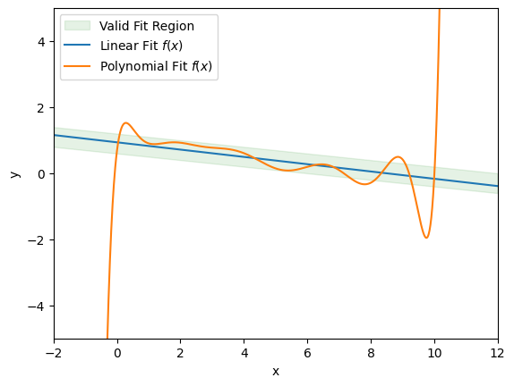
Choosing between two models:

• Consider the following two models fit to the same dataset:

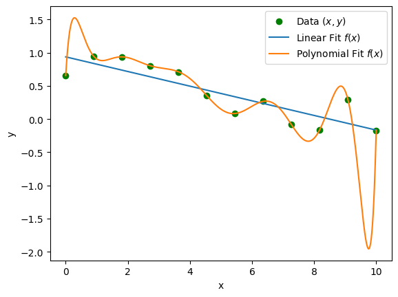
Which model is the more valid model?

• Even though the polynomial perfectly fits the data, it is probably not valid because it extrapolates poorly:

Estimating Validity:

Here's how we can solve the problem of estimating model validity:

• Purposely leave out a random subset of the data that the model is fit to.

  • Use that subset to evaluate the accuracy of the fitted model.

• This subset that we leave out is called the validation set.

• The subset we fit the model to is called the training set.

Training Validation, and Test Sets:

• Common practice is to set aside 10% of the data as the validation set.
• In some problems another 10% of the data is set aside as the test set.

Validation vs. Test Sets:

• The validation set is used for comparing the accuracy of different models or instances of the same model with different parameters.

• The test set is used to provide a final, unbiased estimate of the best model selected using the validation set.

• Evaluating the final model accuracy on the test set eliminates selection bias associated with the accuracies on the validation set.

  • The more models that are compared using the validation set, the greater the need for the test set.

  • This is especially true if you are reporting the statistical significance of your model's accuracy being better than another model.

Preparing Data:

• For each feature vector $\mathbf{x}$, some features vary much more than other features.

• To avoid making our model more sensitive to features with high variance, we standardize each feature, so that it lies roughly on the interval $[-2,2]$.

• Standardization is a transformation $\mathbf{x} \mapsto \mathbf{z}$:

$$z_i = \frac{x_i - \mu_i}{\sigma_i}$$

• $\mu_i$ and $\sigma_i$ are the mean and standard deviation of the $i$th feature in the training dataset.

Exercises: Supervised Learning

• Training, Validation, and Test Sets
• Polynomial Models

Loss functions:

• To evaluate the accuracy of a model on a dataset, we use a loss function.

• A loss function is function of a prediction $\hat{y}$ and a true label $y$ that increases as the prediction deviates from the true label.

• Example (square error loss):

$$E(\hat{y}, y) = (\hat{y} - y)^2$$

• A good loss function should attain its minimum when $\hat{y} = y$.

Model Loss Functions:

• We can evaluate how well a model $f$ fits a dataset $\{(\mathbf{x}_i, y_i)\}_{i=1}^N$ by taking the average of a loss function evaluated on all $(\mathbf{x}_i, y_i)$ pairs.

Examples:

• Mean Square Error (MSE):

  $$\mathcal{E}(f) = \frac{1}{N} \sum_{n=1}^N (f(\mathbf{x}_n) - y_n)^2$$

• Mean Absolute Error (MAE):

  $$\mathcal{E}(f) = \frac{1}{N} \sum_{n=1}^N |f(\mathbf{x}_n) - y_n|$$

For discrete classification problems, we can use the classification accuracy as the model loss:

• Classification Accuracy:

  $$\mathcal{E}(f) = \frac{1}{N} \sum_{n=1}^N \delta(\hat{y} - y) = \left[ \frac{\text{# Correct}}{\text{Total}} \right]$$

Fitting Models to Data:

• Most models have weights that must be adjusted to fit the training dataset:

• Example (1D polynomial regression):

  $$f(x) = \sum_{d=0}^{D} w_dx^d$$

• There are many different methods that can be used to find the optimal weights $w_i$.

The most common method for fitting the data is through gradient descent.

• Gradient descent makes iterative adjustments to weight values such that each adjustment decreases the model loss $\mathcal{E}(f)$.

• Some models (such as linear regression) have optimal weights that can be solved for in closed form.

Review: The Gradient

The gradient of a function $g: \mathbb{R}^n \rightarrow \mathbb{R}$ is the vector-valued function:

$$\nabla g(\mathbf{w}) = \begin{bmatrix} \frac{\partial g}{\partial w_0}(\mathbf{w}) & \frac{\partial g}{\partial w_1}(\mathbf{w}) & \dots & \frac{\partial g}{\partial w_n}(\mathbf{w}) \end{bmatrix}^T$$

• ($\nabla g(\mathbf{w})$ is a function $\mathbb{R}^n \rightarrow \mathbb{R}^n$)

• The gradient at a point $\mathbf{w}$ "points" in the direction in which $g$ increases the most.

• We will use the notation $\nabla_w$ to mean "the gradient with respect to all model weights".

Gradient Descent

• Gradient descent makes iterative adjustments to the model weights $\mathbf{w}$:

$$\mathbf{w}^{(t+1)} = \mathbf{w}^{(t)} - \nabla_w \mathcal{E}(f)$$

Application: Classifying Perovskites

• We will work with some basic classification models that classify perovskite materials as "cubic" or "non-cubic".

Recommended Reading:

• Advanced Regression Models

If possible, try to do the exercises. Bring your questions to our next meeting tomorrow (Tuesday).